Copasetic Flow

I was able to play with the Alcubierre warp drive derivations for a bit today! I'm still trying to absorb all the niceties, but here's what I understand so far. I'm just getting started on all of this and everything is very shaky. So, please, anyone who happens to be familiar with oh, I don't know, the 3+1 formalism of GR say, please feel free to jump in. Actually the more involvement the merrier, whether it be with suggestions, corrections, or questions.

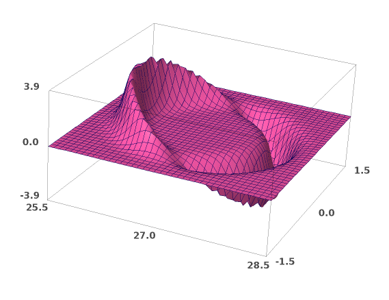
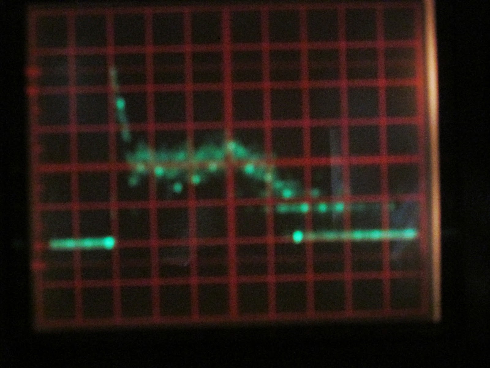
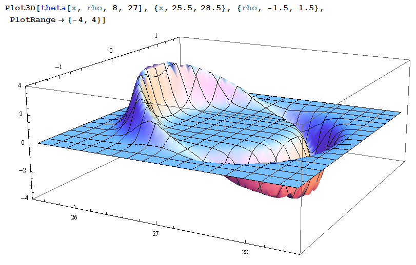
Which brings up the Alcubierre github repository[1]. I went ahead and made an open access github project that for the moment holds only a mathematica file with the derivation details I've been able to compile so far, a wiki, and one open issue, (the space curvature graph looks a little too jaggy). Here's the graph by the way, king of the 'Hello World' moment for Alcubierre work I suppose, (picture 1):

I'd hoped to have more to say about this tonight, but hopefully I can check in again tomorrow when I have a firmer grip on all of this and a bit more coherent one at that, (late night last night).

//Scraggly notes for tomorrow.....
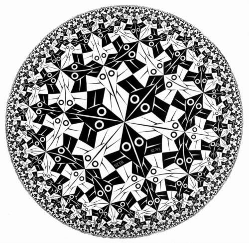
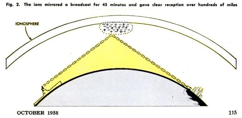
Alcubierre uses a 3+1 formalism. This means that space is assumed to exist in constant time slices, one slice for each instant of time. He furthermore makes space flat. In doing this, he shows that the line element, (the Pythagorean formula for spacetime), indicates that the space will be 'globally hyperbolic' and therefore can't violate causality, in other words, you can't go back in time and prevent your own birth. the way I'm interpreting this is that if I have to move along a hyperbolic path, (picture 2 the red curves are the hyperbolas), in my coordinate system, then I can't execute a close curve, and I can't get back to where I started, (time-wise).

References:
1. github repository
https://github.com/hcarter333/alcubierre

I transferred yesterday's Mathematica file with the Alcubierre warp drive[2] line element and space curvature calculations to the +Sage Mathematical Software System today, (the files been added to the public repository[3]). If you haven't used Sage before, it's a Python based software package that's similar in functionality to Mathematica. Oh, and it' free. I also worked a little more on understanding the theory, but frankly, I made far more progress with the software than the theory. What follows will be a little more of the Alcubierre theory, plus, a cool Sage interactive demo of one of the Alcubierre functions[1], as well as a bit about my first experience with using Sage.

Theory
The theory is fun, but it's moving slowly. Here's the chalk board from this morning's discussion

Alcubierre setup the derivation using something called the 3+1 formalism which means we consider space to be flat, (in this case), slices that are labelled with the advancing value of time. The Greek letters alpha and beta above, are called the lapse, and the shift respectively. The lapse is related to how the spacetime moves from time slice to time slice, and the shift is related to how space changes as time advances.

Understanding the Alcubierre Drive Equations: the shift and the tophat function
When you're cruising across the sky at faster than the speed of light, you don't want to drag too much other stuff with you in your space warp. It's not energy efficient and it just looks silly!

The shift mentioned in the section above is what describes how the ship advances through space and it is a function of the velocity of the moving spaceship. Alcubierre wanted to derive a set of equations that would advance the spaceship through space without advancing anything outside the size of the spaceship. To make sure that the shift moves just the ship and not too much of anything else that happens to be near the ship, Alcubierre tailored the shift function to be very localized in space. Consequently, the shift is the velocity of the ship times a very tophat looking sort of function denoted as f. The tophat ensures that the shift variable is only non-zero and proportional to velocity near the spaceship. In the following equation, r is the distance away from the center of the spaceship, and R is a parameter that should be a little bit large than the ship. Sigma is a parameter that determines how localized the velocity of the spaceship is. You'll see that as sigma increases, the function becomes a nice little square pulse centered on 0 and about the width of the spaceship.

Now here's the really cool thing about Sage. Instead of me just telling you about the function and how it behaves with respect to sigma to become sharper and with respect to R to give you a larger warp for your spaceship, you can actually adjust sigma and R and see for yourself. Voila...[1]. Make sure to hit the button labeled, 'Analyze the Alcubierre tophat function', to start the demo.

My Experience with Sage
Sage rocks! I was able to do everything I'd done with Mathematica, only better! I was also able to publish the demo above with only a little fuss and muss. I'll give you, I haven't learned how to properly size the demo cells yet, but I'll get there I bet. For an example of how to publish Sage demos to the web, just check out the source of this web page. Also, if you want to just play with Sage, please notice that you can type any Sage you like into the code box above. If things become hopelessly intractable, just refresh the page to get back to the original starting point.

Oh, and if you asked if it can make the cool warp graph, well, of course it can!!! Jr.'s into the color pink this month,so here's you're Alcubierre space warp in pink courtesy of Sage!

The Sage Install Experience
If you're using Windows and you want to install Sage to run locally, you're gong to swear a little bit at the gods o' Linux. They've kind of obviously written the documentation pages. However, like me, after you calm down a bit, you'll realize there are only really two steps. First, download the gigantic Sage binary from http://sagemath.org/download-windows.html . It's an ova file, (if you don't know what that is don't worry yet). Next, download VirtualBox and just take all the installation defaults. Select the box that says something like 'Run VirtualBox' as the last installation step. A nice shiny,new GUI will appear asking you which machine you want to run, (this won't make any sense at fit either necessarily). Now, click on the .ova download in your browser. If you're as lucky as Iwas, it will come up in the VirtualBox GUI and just start Sage in your brand-spanking new Linux virtual machine. For a detailed explanation see: http://wiki.sagemath.org/SageAppliance .

References:
1. permalink to blog with the cool demo! (You're here, this is for folks reading outside the blog)

2. Alcubierre's original open access paper
http://arxiv.org/abs/gr-qc/0009013v1

3. Alcubierre Drive Open Science Repository on GitHub
https://github.com/hcarter333/alcubierre

I'm taking a little break from the Alcubierre work[1] and jotting down a few notes on how to embed +Sage Mathematical Software System cells into html pages. I couldn't find any documentation or howto pages for this, so here are my instructions for the next time I get ready to do this.

Insert Sage Javascript at the Bottom of the Page
For whatever reason, my blogspot entries will erease code placed at the top of a post. They will however allow scripts that are included at the end of the page, go figure. So, at the bottom of the page place the following html code:

<script>
$(function() {
sagecell.makeSagecell({
inputLocation: '#graphdemo',
evalButtonText: 'Analyze the Alcubierre tophat function'});
});
</script>

In the position on the page where you want your actualy sage cell to be displayed insert a div wrapping your sage code like so


<div id="graphdemo">
<script type="text/code">
ftophat(s,r, R)=((tanh(s*(r+R)))-(tanh(s*(r-R))))/(2*tanh(s*R))
ftophat(s,r, R)=((tanh(s*(r+R)))-(tanh(s*(r-R))))/(2*tanh(s*R))
@interact
def _(sigma=(1..23), R=(1..7)):
  ftp = ftophat(sigma, r, R)
  pt = plot(ftp, -R-1, R+1,color='blue', thickness=2)
  html('$f(r)\;=\;\dfrac{tanh(\sigma(r+R)) - tanh(\sigma(r-R))}{2 tanh(\sigma R)}$')

  show(pt, ymin = -0.1, ymax = 1.1)</script></div>

You can choose the div id to be anything you want, however, it needs to match the text for inputlocation in the scripting block. Within the <script type="text/code> tags, put whatever Sage code you'd like to demonstrate on your web page. Finally, place the text you want displayed on the blue button that will start the Sage cell in the evalButtonText field of the Javascript block. For a page that demonstrates all this, see the latest Alcubierre demo on this site. That's all there is to it! Please let me know if you have any questions or ideas. By the way, does anyone know how to specify the size of the Sage demo block on the html page? Mine exceeds my page width and turns on scroll bars.

References:
1. Alcubierre work
http://copaseticflow.blogspot.com/2014/06/the-alcubierre-warp-drive-tophat.html

Lab Book 2014_06_20 Hamilton Carter

New to the lab book? Scroll to the bottom for background and a summary of the experiment.

Pulling the Dewar from the Table

The spray Styrofoam was shaved off the Dewar this morning revealing that the Dewar had originally been installed on a piece of regular Styrofoam and the spray coating was added later

The plan is to peel away as much of the spray foam as is practicable, and then do a two person lift of the Dewar out of the table. The Dewar will be immediately placed in a padded box.

The Dewar was successfully removed! Next, I’ll remove the shelf and put the magnet in place. There’s one cooling tube that was knocked off the magnet as it turns out, so that will have to be fixed.

Vacuum Pump Down!

The leak detector vacuum pump appears to be broken. The reading on it is a much worse vacuum than from the auxiliary one on the lower shelf of the cart


Leak Detector Pump	Auxiliary Pump

The pump was tested using a thermocouple gauge system shown below. The actual vacuum detector has a blue label is attached to the OCF brass flange. The flange isn’t visible as it is enclosed in the larger black plastic clamp.

The detector cable plugs into a readout box:

The flange was attached directly to the mechanical roughing pump that was being tested by first detaching the hose between the mechanical and the diffusion pump at the diffusion pump end and then inserting the assemblage shown attached to the gauge above into the hose as shown below

I’m wondering how much work it would take to put our thermocouple vacuum meter on an Arduino data capture system, hence the digital voltmeter in the second picture to check the voltages that are available and should be somehow related to the vacuum reading on the meter.

Background

Hirsch's theory of hole superconductivity proposes a new BCS-compatible model of Cooper pair formation when superconducting materials phase transition from their normal to their superconducting state[1]. One of the experimentally verifiable predictions of his theory is that when a superconductor rapidly transitions, (quenches), back to its normal state, it will emit x-rays, (colloquially referred to here as H-rays because it's Hirsch's theory).

A superconductor can be rapidly transitioned back to its normal state by placing it in a strong magnetic field. My experiment will look for H-rays emitted by both a Pb and a YBCO superconductor when it is quenched by a strong magnetic field.

This series of articles chronicles both the experimental lab work and the theory work that’s going into completing the experiment.

The lab book entries in this series detail the preparation and execution of this experiment… mostly. I also have a few theory projects involving special relativity and quantum field theory. Occasionally, they appear in these pages.

Call for Input

If you have any ideas, questions, or comments, they're very welcome!

References

1. Hirsch, J. E., “Pair production and ionizing radiation from superconductors”, http://arxiv.org/abs/cond-mat/0508529

The Alcubierre drive works, (theoretically), by warping space 'downwards' in front of a spaceship and 'upwards' behind it, (picture 1).

The net effect is that the spaceship always feels like it's free-falling through space. We have to be careful not to let the spaceship approach either the upward or downward walls of the curved space shown above. In these regions, gravity due to the curvature of space is changing rapidly, and will cause uneven forces, known as tidal forces, on different portions of the spaceship that can cause it to break apart. That's where Alcubierre's tophat function comes in. The tophat is the input to the operation that describes how space is warped by the drive. It's nice, flat top becomes the flat area in the middle of the warp shown above where the spaceship can safely rest.

In case you weren't there, here's the description of the tophhat function I provided in the last post on the Alcubierre drive[1], (stay tuned after the rehash for an explanation of the math behind the warp moving through space):

"The shift mentioned in Alcubierre's formulas[2] as beta describes how the ship advances through space and it is a function of the velocity of the moving spaceship. Alcubierre wanted to derive a set of equations that would advance the spaceship through space without advancing anything outside the size of the spaceship. To make sure that the shift moves just the ship and not too much of anything else that happens to be near the ship, Alcubierre tailored the shift function to be very localized in space. Consequently, the shift is the velocity of the ship times a very tophat looking sort of function denoted as f. The tophat ensures that the shift variable is only non-zero and proportional to velocity near the spaceship. In the following equation, r is the distance away from the center of the spaceship, and R is a parameter that should be a little bit large than the ship. Sigma is a parameter that determines how localized the velocity of the spaceship is. You'll see that as sigma increases, the function becomes a nice little square pulse centered on 0 and about the width of the spaceship".

Here's the sage demo of the tophat function's sigma and R parameters effect it:

You may have noticed that the all the graphs of the tophat function have been in terms of r, and not our usual spatial axis, x. The value of r itself is another mathematical function defined by Alcubierre. The value of r is the distance away from the center of the spaceship at a given point in space. r is defined as:

$r(x_s) = \sqrt{(x-x_s)^2+y^2+z^2}$

For our example we're setting x and y to zero, so that we only move along the x direction. With this simplification, we get

$r(x_s) = (x-x_s)$

OK, that leaves us with the question, what is $x_s$ ? $x_s$ is the trajectory we want the ship to travel along with respect to time, something like this:

In other words, suppose we want to move from the location $x=0$ to the location $x=17$, then $x_s$ will take the values 1 to 17 as time progresses. For our example below, we're going to assume time progresses in a uniform fashion and we advance one unit in x for each time tick.

Now, if we graph what's going on in terms of space, (the x variable), instead of terms of r, (the displacement from the spaceship), we get a different, and moving picture for the tophat function which is now:

$f_{tophat}\left(r\left(x_s\right)\right) = \dfrac{tanh(\sigma((x-x_s)+R))-tanh(\sigma((x-x_s)-R))}{2tanh(\sigma R)}$

Let's call this a chained function, (since it will fit in nicely in the next post where we'll use the chain rule for taking derivatives to get the curvature of space caused by the warp drive). The position value returned by the trajectory for each instant of time is fed to the formula r which is fed to the tophat function. And...

by stepping the value of our trajectory, $x_s$, from 1 to 17 as discussed, we get a moving tophat function that travels along the path we want to move through in space. We're not all the way to the warp function yet, that'll be next time.

The animation above was created with sage. As of yet, I haven't been able to get animations to work in an embedded sage cell, but for those who would like to play with the math, here's the sage code:

ftophat(s,r, R)=((tanh(s*(r+R)))-(tanh(s*(r-R))))/(2*tanh(s*R))
fhts = [plot(ftophat(23, x-xs, 1), (1,17), color=Color(0,0,0), ymin=-0.1,ymax=1.1,xmin=0,xmax=18) for xs in sxrange(2.1,17,.2)]
b = animate(fhts) b
b.show()

The code has also been placed in the github repository[3].

References:

1. Previous post on the Alcubierre drive
http://copaseticflow.blogspot.com/2014/06/the-alcubierre-warp-drive-tophat.html

2. Alcubierre's paper:
http://copaseticflow.blogspot.com/2014/06/the-alcubierre-warp-drive-tophat.html

3. github repository:
https://github.com/hcarter333/alcubierre

I spent most of yesterday travelling between Austin and College Station, but I did manage to get a little bit of research in. I'm looking for other experiments related to Hirsch's theories we can do in conjunction to the search for H-rays. One of the measurable predictions of Hirsch's theory is a change in the coefficient of sliding friction when a material enters it's superconducting state.

All about friction[6]

New to the lab book? Scroll to the bottom for background and a summary of the experiment.

Hirsch mentions[1] that a finding of reduced friction in superconductors might be evidence in support of his hole theory of superconductivity.

Furthermore, the electronic layer outside the surface
is likely to affect the friction properties of the superconductor,
by providing a ‘lubricating layer’ on top
of which another material would slide. As a matter of
fact, an abrupt drop in sliding friction between a lead
surface and solid nitrogen has been observed when Pb
enters the superconducting state [15]. We infer that
this effect is due to the physics of the electron layer
outside the surface discussed here, and hence that a
friction drop should be observed for all superconductors.

He cites, ([15] above), an experiment reported by Dayo, Alnasrallah, and Krim[2] as having actually shown a drop in the sliding friction between Pb and solid nitrogen in a liquid helium reservoir. The experimental setup for the DAK experiment is shown in picture 2.

A quartz resonator was covered with thin film of Pb and then nitrogen was adsorbed into the surface of the Pb. By measuring the quality factor of the underlying quartz resontaor, the researchers claimed they were able to monitor the friction between the Pb and the layer of nitrogen. If the nitrogen could easily slide across the Pb, then the underlying resonator could vibrate more easily than if it could not. This apparatus described has been used freqently in friction research and is know as a quartz crystal microblalnce. DAK reported that when the Pb entered it's usperconducting state, there was a large, almost discontinuous, reduction in the coefficient of sliding friction between the Pb and the nitrogen.

There are issues however... Renner, Rutledge, and Taborek, repeated the DAK experiment and got a null result. Krim replied stating that the RRT experient had used a contaminated sample. The important takeaway for the work here is that if Krim is correct, then additional friction experiments would require more resources than we currently have at hand.

A similar test has been done with YBCO, by Krim and Altfeder[5]. The results showed that there was a roughly linear reduction between YBCO and a Fe surface as the temperature of the YBCO approached the critical temperature, but that friction held steady once the YBCO entered the superconducting state.

References

1. Hirsch on superconductors and friction [open access]
http://arxiv.org/abs/cond-mat/0301611

2. A. Dayo, W. Alnasrallah, J. Krim, Phys. Rev. Lett. 80 (1998)
1690.

3. More theoretical work on the DAK experiment
http://arxiv.org/abs/cond-mat/9905264

4. R. L. Renner, J. E. Rutledge, and P. Taborek, preceding
Comment, Phys. Rev. Lett. 83, 1261 (1999).
http://journals.aps.org/prl/abstract/10.1103/PhysRevLett.83.1261

5. YBCO and friction
http://scitation.aip.org.lib-ezproxy.tamu.edu:2048/content/aip/journal/jap/111/9/10.1063/1.4717983

6. Friction on Wikipedia
https://en.wikipedia.org/wiki/Friction

Background

Call for Input

If you have any ideas, questions, or comments, they're very welcome!

References

1. Hirsch, J. E., “Pair production and ionizing radiation from superconductors”, http://arxiv.org/abs/cond-mat/0508529

+Jonah Miller is currently working on a multi-part series of articles on how computers work. In one of the installmetns he mentioned the good old triode vacuum tube with a cathode, plate, and grid. That brings up the subject of today's post, the grid dip meter, (GDM). If you wandered over here from the ham radio practice tests[1], and you want the shortest answer possible, then click here, or scroll down the page. If you want more information, read on:

The grid Dip meter schematic is shown in picture 1.

The main purpose of the circuit, at least for amateur radio operators, is to determine the resonant frequency of some other circuit or device, (like an antenna). Let's say you've built you're latest radio and you'd like to get all the power you can from the driving finals, into the antenna. To do that, you'd like to make sure that the antenna resonates at the same frequency you'd like to send and receive at. If the antenna resonates at a little bit lower frequency, you can always trim it's length, or if it oscillates at a little bit higher frequency, you can always make a longer one. To find out which I need to do, I'll use my grid dip meter to determine the antenna's resonant frequency.

The basic grid dip meter's circuit consists of a Colpitts oscillator with the inductor, L1, of the LC feedback loop exposed and protruding from the device, (see picture 2), it's the coil on the far left edge of the picture.

To determine my antenna's resonant frequency, I'll attach a small coil to the middle of it, (I tend to only use dipoles because I'm lazy). Next, I'll place the exposed coil of the grid dip meter near the coil attached to my antenna. Then, I'll tune the oscillator's operating frequency until I see the reading on the meter on the front face of the apparatus, which is denoted by G in the schematic, dip, (hence the name).

So,why does the current being supplied to the grid of the Colpitt's oscillator dip? At the resonant frequency of the device being measured, the magnetic field from the inductor begins to drive the coil on the device under test. In this case, the antenna radiates that energy away. The current that was driving the grid is now reduced in an amount related to the amount of energy that went into the device under test, (the antenna). Pretty cool!

The Answer to the Ham Radio License Exam Question
You want the two coils to be as loosely coupled as possible. If they are tightly coupled, (located very close to one another), then the inductance in the coil attached to the device under test will effect the resonant frequency of the GDM. The end result will be that the resonant frequency won't be the actual resonant frequency of the device under test, it will be an odd munge of the device and the GDM circuit. On the flip side, you don't want to couple too loosely either, or the grid current simply won't dip.

A Year and a Month Ago

Radiating Superconductors, Arduinos, and Data Acquisition
http://copaseticflow.blogspot.com/2012/06/radiating-superconductors-arduinos-and.html

LabBook 2014_05_26 Superconductor Quenching Magnet Chilling Supply and Leak Detector Testing
http://copaseticflow.blogspot.com/2014/05/labbook-20140526-superconductor.html

References:

1. http://copaseticflows.appspot.com/hamtest

Imagine living thousands of years ago in ancient Sumeria as a mathematician. Your medium for storing infomration is cuneiform on clay tablets. As you work, you stamp each equation into wet clay by making wedge shaped marks using the blunt end of a reed to make a finished document that looks like this (picture 1)[1]

When your instructor tells you to investigate the properties of a table of let's say, a hundred numbers or so, you might sigh in resignation, and plan on having results by sometime next week.

With the advent of paper and pencil, things become much easier. There's still lots of work to be done, but the recording of the information so that it can be viewed and worked with is, comparatively speaking, a piece of cake.

Finally, though, the computer comes along and getting a table of 100 numbers is more like playing. With +The SageMathCloud the 100 number task suggested in the +Mathematical Association of America video below can be done easily by anyone with a web browser. Watch the video[2] and then read on for an example of just that.

The problem is to figure out the maximum slope, a, for a line described by y = 2 + m*x where 1/2 < m < a. The game is that the line cannot intersect with any lattice points. These are points where the x and y coordinates both have integer values. The first minute or so of the video has a great illustration of this. So, we don't want to hit any of the blue lattice points shown in picture 2 as we crank up the slope of the line to the value m < a.

Dr. Tanton suggested that we take a look at the value of the line with slope m = 1/2 and how far it was from each of the lattice points directly above it out to the x coordinate of 100. Here's the graph of the m = 1/2 line as well as the lattice points that we need to avoid as we crank the slope up from 1/2. (picture 2)

and, here's the sage code if you'd like to play with it

Now, instead of figuring out the slope that would hit each successive 'bad' lattice point, we can have Sage do it for us, and dump it out as a list of slopes at each point. Cick the blue button below for the table of slopes necessary to just hit each lattice point. In other words, by staying less than each successive slope, we can just miss that lattice point.

We see that the slope which will hit the 99th lattice point we're trying to miss is 50/99. So, in the problem as asked, the maximum the slope, a can be is a < 50/99.

Another snazzy thing we can look at is how the maximum slope progressed as we went from lattice point to lattice point out towards 99. Here's the graph: (picture 3)

Here's the Sage code used to generate it. Remember you can modify the sage code in any of these cells and hit the blue button again to find out what effect your modifications had.

References:
1. http://books.google.com/books?id=i-juAAAAMAAJ&pg=PR3#v=onepage&q&f=false

2. Video
http://youtu.be/j2J6NEGTMsY

Penrose created visually appealing and conceptually utilitarian conformal maps of spacetime including the point at infinity for general relativity.
Penrose published his first articles on diagrams with his dad, L.S. Penrose. The article cited an M.C. Escher exhibit Penrose attended in 1954
Roger Penrose wrote over 20 books and articles referencing Escher. You can find them all on Google Scholar
When Penrose and Penrose published their first article citing Escher’s work, he hadn’t created his woodcuts of the hyperbolic plane which illustrate a conformal infinity. By 1962 when the first Penrose diagram, (a conformal map with infinity), appears, Escher had, (1959).
Escher’s woodcut is included in Penrose’s book “The Road to Reality”, and is very similar in form to Penrose’s first published conformal map of the point at infinity in spacetime.
There’s an entire collection of videos featuring Roger Penrose.
Penrose used Escher’s “Waterfall” to illustrate aspects of Bell’s non-locality work.
This list was inspired by Aaron Wright’s recent article in Endeavour. It’s not open access, but if you’re near a university library, here’s the link. Aaron’s other article on this subject isn’t open access either, but that’s OK as both articles’ are nicely summarized in one of Aaron’s blog posts.
Aaron is also a photographer. http://photo.aaronswright.com/ The picture shown here is my favorite so far.

References:
1. Aaron Sidney Wright, The origins of Penrose diagrams in Physics, Art, and
the Psychology of perception, 1958–62, Endeavour, 37, (2014), 133
http://dx.doi.org/10.1016/j.endeavour.2013.02.001

2. Penrose Diagrams in PRL
http://journals.aps.org/prl/abstract/10.1103/PhysRevLett.10.66

3. Escher Bats 1960
http://www.mcescher.com/gallery/recognition-success/circle-limit-iv/

4. Escher Fish 1959
http://www.wikiart.org/en/m-c-escher/circle-limit-i

5. Penrose diagram first mentioned in t1962 at a conference in Warsaw Poland
Roger Penrose, ‘‘The light cone at inﬁnity,’’ in Conference internationale sur les
the´ories relativistes de la gravitation: Sous la direction de L. Infeld, ed. L. Infeld
(Warszawa: PWN–Editions Scientiﬁques de Pologne, 1964), 369

6. First Penrose diagram in PRL in 1963
Roger Penrose, ‘‘Asymptotic properties of ﬁelds and space-times,’’ Physical Review
Letters, 10 (2) 1963, 66–68.

7. Penrose and Penrose cites Escher exhibit
L. S. Penrose and Roger Penrose, ‘‘Puzzles for Christmas,’’ New Scientist (Dec.)
1958, 1580.

8. Additional Penrose and Penros article
L. S. Penrose and Roger Penrose, ‘‘Impossible Objects: A Special Type of Visual
Illusion,’’ British Journal of Psychology 49 (1), 1958, 31.

9. Penrose on Escher in 1992
http://www.jstor.org/stable/1575844

10. Escher Waterfall
http://www.mcescher.com/gallery/recognition-success/waterfall/

Summary

Callibrtion of the NaI gamma ray detector has begun. A mistake in the gain and treshold settings made it appear as if the dectector might not be working properly as it gave the same energy spectrum with and without a Cesium 137 source present. Once the gain and threshold were properly set what appeared to be good spectra were recorde.

New to the lab book? Scroll to the bottom for background on the experiment.

Using the Photomultiplier Tube power supply

First, turn on the lever switch labeled “Power” on the lower left hand side fo the box. Make sure to wit fo rhte “Stdby Reset” panel light to illuminate before switching on the “High Voltage” lever switch

To turn on the QVT, switch on the power switch on the NIM Bin supply on the far right hand side of the bin.

Clearing the QVT

To clear the contents of the QVT, hold the start/stop switch in the stop position while toggling the clear switch.

picture 1 and 2 are the front panel and the cleared spectrum

Spectrum Readings

Taking a reading with the Cs 137 source directly against the side of the NaI crystal. The following picture shows the setup.

The recorded spectrum follows.

The printer was used to capture the data for keypunch purposes

Here’s the graph of the spectrum from the printed data

After 35 minutes and 23 seconds, I wound up with a very similar spectrum with no source.

Oscilloscope settings used to record spectra.

The spectra with and without the source appear to be very close to identical.

Ideas:

· Try with a different source

· Try with attenuation to see if the peak moves, (it should)

New information: the observed peak is the pedestal of the detector. The gain on the PMT was not turned up high enough to see the signal from the source. Consequently, whatever noise wsacoming in wasbeing integrated by the QVT and displayed in the lower channels from channel 153 on up. The threshold was also set too high which is why the channels below 153 are empty.

To calibrate the photon energy displayed by each channel, I’ll recordth eknown energies of three source, Cs 137,Co 60,and Sr 90. Using these points, alinear inrepolation of energy per channel will be made

The gate on the QVT determines how long the device should integrate charge signals before allocating them to a counting the appropriate energy channel. The gate width can be read from a test point on the front panel of the QVT. The QVT waits for a signal that exceeds the internal trigger voltage and then integrates the signal for an amount of time defined by the gate width.

The gate signal at present is… 0.35 uS.

Threshold was also set on the front panel and was set for -3.41 Volts initially. The value read on the threshold test point is multiplied by 100. The new value is -1.49 Volts.

The PMT has been biased with 2600 Volts this afternoon and was at 2000 Volts when the two spectra were taken this morning.

The QVT records one quarter picoCoulomb perchannel. By looking at the raw pulses on the scope, and considering the 50 ohm termination, you can caluculate how many coulombs you have.

There is currently a factor two attenuation. It’s in so that we can get all the lines on the same specturum. The attenuation lets you find out the entire spectrum from the biggest to the smalles t nd then once you know where things are you can find the soure.

Thers a peak on the right hand edgefrom frobblay the concrete which would be Potassium 40.

The shield will prevet the potassium 40 peak.

Read up o the quarters I the QVT manual to see what they do. Anoterh way of getting bigger sigals is to raise the voltge on the PMT.

The last picture on the camera is the newest spectrum.

Measure the present threshold in the morning. DONE

Background

Call for Input

If you have any ideas, questions, or comments, they're very welcome!

References

1. Hirsch, J. E., “Pair production and ionizing radiation from superconductors”, http://arxiv.org/abs/cond-mat/0508529

Summary:

Much more plunking around with the NaI detector and sources today. A Pb shield was built to eliminate cosmic ray muons as well as potassium 40 radiation from the concreted building. The spectra are much cleaner, but still don't have the count rates or distinctive peaks that are expected.

New to the experiment? Scroll to the bottom to see background and get caught up.

Lab Book

Threshold for the QVT is currently set at -1.49 volts. Remember to divide this by 100 to get the actual threshold voltage.

A new spectrum recording the lines of all three sources, Cs 137, Co 60, and Sr 90, was started at approximately 10:55.

Took data for about an hour.

Started the Cs 137 only spectrum at about 11:55 AM

Here’s the no-source background from yesterday

In comparison, here’s the 3 source spectrum from this morning.

The three source spectrum shows peak structure not exhibited by the background alone.

I forgot to take scope pictures of the Cs137 run. I do however, have the printout, and will enter the data soon.

A Pb brick shield was built to calm down the background noise from cosmic ray muons, concrete K 40, and radon.

The source is situated at the base of the NaI crystal as shown below:

The spectrum from a Co 60 source in the Pb bunker is shown below. I’ll get the data entered soon.

The photo quality is poor, but I believe there’s a peak in the middle of the screen.

Finally for today, here’s the spectrum with the Pb bunker and no source. Note that it’s much cleaner.

I've played one other trick here by using the linear output as opposed to the log output that was used in all the other plots. It makes the spectrum appear more clean.

Background

Call for Input

If you have any ideas, questions, or comments, they're very welcome!

References

1. Hirsch, J. E., “Pair production and ionizing radiation from superconductors”, http://arxiv.org/abs/cond-mat/0508529

You might remember one of my G+ posts[2] from a few months ago, about a video wherein a Soviet astronaut spun a small wingnut,

OK, so not the Teenage Mutant Ninja Turtles character, an actual wingnut[3]:

+Bruce Elliott pointed out in a comment to the original post, (see below), that rotating an object, like a book, about its intermediate axis, (an axis parallel to the bottom edge of the cover), will cause unstable rotation.

Now, Brian Weinstein of The Fouriest Series[1] has posted a mathematica demo complete with gifs of the rotating book. On top of that, he includes a link to a gist that contains the Mathematica code[4] for creating the rotation demo.

Here's the rotating book image from Brian's page, which I'd advise following if you enjoy mathy gifs!

G+ post mentioned above

References:
1. Awesome intermediate rotation page
http://fouriestseries.tumblr.com/post/91685028535/rotational-stability

2. G+ post
https://plus.google.com/108242372478733707643/posts/KxN4Dj55a7E

3. Wingnut video
http://youtu.be/dL6Pt1O_gSE

4. Mathematica code gist
https://gist.github.com/BrianWeinstein/6a8a852c46053c0c8d7d

Summary:

The photomultiplier tube on the NaI detector doesn't seem to be doing quite what it should. There's a generally held belief, (when I say generally held belief, read, "a professor told me"), that the count rates aren't high enough. Last week, the case of the tube was arcing to my hand making nice little static shock looking flashes of light. Consequently, I spent today doing research on the three most likely PMT tubes that are housed within the detector. Since the tube is surrounded by a mu metal magnetic shield, it can't be inspected to find it's exact type. I have a call in to the company that purchased the original manufacturer, and hopefully they can figure out which kind of tube we have. In the mean time, I've turned down the tube bias which seems to have stopped the arcing. I've also inspected the voltage divider that provides the accelerating potential for the dynodes in the PMT. This inspection could just as easily have stopped the arcing by moving a component away from the metal housing. While the divider chain case was off I went ahead and drew a schematic of the circuit. A partial Cesium137 spectrum was taken this afternoon and it looks promising.

New to the experiment? Scroll to the bottom to see background and get caught up.

Lab Book 2014_07_14

Lab Book 2014_07_14 Hamilton Carter

I’m working on debugging the dynode divider which appears to have been damaged last week, probably by running too much voltage on the power supply attached to it. I came across the following spectrum that looks great given the nature of the spectra that may be present in the experiment. The prediction of the maximum possible radiated energy via h-rays does not mention anything about what the overall spectrum will look like. If we have a maximum energy of 187 keV, we could also get radiation anywhere below that level. In the following spectra from the Harshaw manual, you can see that the exact detector that is to be used can see radiation all the way down to the 32 keV Barium K X-ray line.

I found a thesis where the Harshaw 12S12/E was used. We have a 12S12/3. I’m not sure how they’re related yet. In the thesis, a Dumont 6363 photomultiplier tube was used. There is also a schematic for the dynode voltage divider chain that was used with the Dumont 6363.

I’ll check these resistor values against the ones in the dynode divider if necessary. I found a second thesis that mentions using a supply voltge of 900 rather than the 1000 Volts mentioned in the first thesis, (see the figure above).

I also found a paper that mentions the Harshaw 12S12/3 specifically. The is the model that we have. The paper mentions another key piece of information. The aluminum housing of the crystal is 0.5 mm thick and is made of spun aluminum. The window itself if listed as 0.010 inches thick at another web site.

Here, the potential is listed as 660 V.

On a mostly side note, this report is kind of interesting as to what is available for history of physics research. It’s the equipment inventory for a nuclear rocket project performed by General Aerojet.

In this report, the PMT is listed as a RCA 8054.

In this LANL report written by Ellery Storm, the PMT is also listed as an RCA 8054.

This might be a good reference for supplementing with film detectors. It was authored by Ellery Storm.

http://www.osti.gov/scitech/biblio/4399073

Resistor color code tool used to check resistor values:

http://www.digikey.com/en/resources/conversion-calculators/conversion-calculator-resistor-color-code-4-band

Source mentioning that tube is in apparatus	Tube Type	Max Anode/ Cathode Voltage	Max Consecutive Dyn V
Harshaw Manual	4524	2500 V	300 V
	8054	2000 V	250 V
Harshaw Manual	Dumont 6363	1800 V	Not specified

The following pictures detail what the voltage divider chain being used to drive the PMT looks like:

This one details the high voltage input and its associated 55.6 ohm resistor.

This is a side view of the same input. The identical resistors shown in the foreground are part of the dynode voltage divider chain, see the schematic below.

This picture continues along the divider chain. Note the capacitors that are connected in parallel across the last few dynode resistors. They are omitted in the hand drawn schematic below.

Finally, the green wire connects the plate/anode of the PMT to the pulse output that is used by the QVT.

A hand drawn schematic of the divider chain follows:

The pinouts of both RCA tubes and the DuMont tube are all identical and can be seen below.

Dumont Pinout

RCA Pinout

I setup the detector to take yet more data on the Cs 137 source this afternoon. I’ll have the data in the morning. Here’s what the spectrum was up to when I left for the evening.

The key difference here is that the tube is biased to 2000 V instead of 2600 V. The arcing from the tube to my hand has stopped at this bias voltage.

The spectrum looks like it is already exhibiting two peaks after an hour or so of taking data.

Finally, a spreadsheet was made to calculate the voltages on the dynodes. A sample output is shown below.

References:

These are some of the original source links for the reports mentioned above. Since Word tries to open pdfs in Explorer instead of Chrome, all the links in the text are to Google Drive locations.

Ellery Storm report

http://fas.org/sgp/othergov/doe/lanl/lib-www/la-pubs/00365209.pdf

I thought I remembered the name Ellery Storm and it turns out he wrote a book of stories about New Mexico.

Harshaw Manual

https://drive.google.com/file/d/0B30APQ2sxrAYMFV4UWE2VXRTOGc/edit?usp=sharing

RCA 8054 manual original site:

http://frank.pocnet.net/sheets/049/8/8053.pdf

Background

Call for Input

If you have any ideas, questions, or comments, they're very welcome!

References

1. Hirsch, J. E., “Pair production and ionizing radiation from superconductors”, http://arxiv.org/abs/cond-mat/0508529

There's an ongoing effort to save HAARP from the demolition block[4], and as it inevitably does in all matters HAARP, the topic of chemtrails came up. Chemtrails are by and large considered to be an urban legend, but like all good legends, it turns out there's more than a trace of truth embedded in the story Perhaps the chemtrail legend has propagated so well because the ham radio community at large was involved in the first experiment that might have blossomed into the chemtrail mythos. During a magical period, in the mid '50s the United States Air Force experimented with augmenting the performance of the ionosphere, (think HAARP), by creating airborne clouds of particulate reflectors, (think chemtrails).

In his landmark 1958 article describing the experiment[1], author Michael Gladych, (expect to see more about Gladych in these pages soon), first explained what the ionosphere was, first in words:

"In this electronic age, everybody knows that the ionosphere is an electrified upper atmosphere region that bounces off radio waves around the globe."

and then with a picture:

Gladych went on to explain that the reflectivity of the ionosphere was due to rays from the sun ionizing molecules of the atmosphere forming a conducting layer between 60 and 70 miles up. As many ham radio operators know, this reflecting layer is a boon to radio communications in the high frequency range around 7 MHz, but higher frequencies like microwave communications at 144 MHz are not reflected back to Earth. However, there are periods of intense solar activity that improve the 'reflectivity' of the ionosphere. For more about this, see +Ian Poole's excellent article on sunspots and the ionosphere.

What the Air Force sought to do was create these enhanced ionospheric patches at will. They assembled a team of researchers in Bedford Massachusetts, Dr. Frederick F. Marmo and his associates L. Aschenbrand, and J. Pressman. Marmo and company reasoned that by creating an easy to ionize cloud, one made out of particulate phosphorous, they could deliver an ionosphere in a can. And thus was born Operation Smoke Puff.

A launch pad for an Aerobee rocket was assembled in southern New Mexico, and a fifteen pound, (xxx kilo), clump of phosphorous was launched to an altitude of 60 miles where it was detonated. Ham radio operators in a radius of 700 miles around the launch site were asked to transmit on frequencies between 7 and 144 MHz and submit reception reports on the quality of their communications. Sure enough, the artificial ionosphere worked like a champ providing "next-door clear" communications for 45 minutes.

It Seemed Like a Good Idea at the Time
As it turned out, the 45 minute dispersion rate was a bit limiting, and there were other problems besides. The invention only worked during daylight hours when there was sunlight available to ionize the cloud. There were plans in the works for a night enabled version, but it had it's own issues. While it was advertised as being very effective at confounding enemy radar, the cloud presented a bit of a defensibility problem in that it would have produced a visible light glow over the ground target it was protecting, easily pointing out its location for bomber pilots. In the ever-optimistic 50's though, there was still an upside. Gladych reported that

"for peacetime applications, the glow of a large and longer-lasting ion cloud could be used to illuminate a city better than the street lamps.

References:
1. Gladych's article in Popular Mechanics
http://goo.gl/gZ72AR

2. +Ian Poole article on sunspots and the Ionosphere in Radio Electronics
http://www.radio-electronics.com/info/propagation/ionospheric/sunspots-cycle-activity.php

3 Marmo's patent on expansions to the Operation Smoke Puff work
http://www.google.com/patents/US3052052

4. Saving HAARP... You know, for the hams...
http://chipdesignmag.com/carter/2014/07/16/help-save-haarp/

5. Newspaper article about operation Smoke Puff 4/18/1957
http://news.google.com/newspapers?nid=1314&dat=19570418&id=u7YyAAAAIBAJ&sjid=OecDAAAAIBAJ&pg=2136,371543
mentions Dr. O. G. Villard of Stanford who headed up the radar measurements of the cloud.

6. Popular Electronics article enlisting listeners
http://www.americanradiohistory.com/Archive-Poptronics/50s/57/Pop-1957-06.pdf

also shown here:

7. O.G. Villard on Operation Smoke Puff
http://www.americanradiohistory.com/Archive-Radio-News/50s/Radio-News-1957-06-R.pdf

Summary: I'm still checking and re-checking the NaI detector. I've yet to get a reliable spectrum out of it, but last night's run at least has distinguishable peaks. The company that made our detector 50 years ago believes that we probably do have an RCA 45xx series photomultiplier tube which would mean that the 2400 V bias I have to drive the tube at to get a signal is actually OK. The 45xx series has a maximum bias voltage of 2500 V.

If you're new to the experiment, scroll to the bottom for background.

The Cs137 spectra that was started at 3:13 PM yesterday was ended today at about 9:50 AM. The photo of the spectrum follows

There are a number of oddly shaped peaks that may ben been created by channel overflow now that I think about it. The data was printed and the linear chart is shown below:

If I ‘fix’ the supposed channel overflow by adding the value of the full register back in to the count, on the first step I get:

Which fixes the two peaks to the right, but not the one to the left.

Working under the assumption that the register overflowed twice in this region, I added in two full register counts to these data points and wound up with

We may be able to assume that the two non-plateau peaks are the two peaks associated with Cs 137. I’m running a Co60 spectrum now and should have results by the end of the day.

Here’s a picture of the Cs137 sectrum again for reference.

Hunh, Cs137 only has one noticeable peak, or at lest one peak that should be larger than all the rest. I've been told that our detector shouldn't be able to see the 32 keV line to the left of the graph.

Background

Call for Input

If you have any ideas, questions, or comments, they're very welcome!

References

1. Hirsch, J. E., “Pair production and ionizing radiation from superconductors”, http

Picture 1 is taken from Villard's report[5] on long delay echoes (LDEs)

There's lots of science out there still to be done, even in age old hobby of ham radio. In one of my recent posts, I talked about Operation Smoke Puff, and experiment that bounced radio signals off a man-made cloud of ions to a distant receiver. The project was sponsored by the military with hopes of being able to provide longer distance radio communications by creating a made-to-order skip path. As it turns out, radio signals and the ionosphere are quite capable of providing long distance communications paths all by themselves, for folks who don't happen to own a missile launcher. In some cases, a signal can be made to transmit around the entire planet. Many amateur radio operators have experienced the phenomenon of round-the-world radio skips where the transmitted signal continues to bounce, completing a path that spans the globe and arrives back at the station. The radio operator winds up hearing their own transmissions a fraction of a second after it was sent. But, what about signals that take seconds to arrive back at their origin? Where did they go in the meantime?

Round-the-world transmissions were well understood before the 1927, when a ham reported a propagation mode that we have yet to understand. Carl Stormer reported hearing his own signal in his headphones about a seventh of a second after it was transmitted. That's fairly normal, it's just an around the world signal as described above. What Stormer didn't expect was hearing his own signal again a few seconds later. While several hypothesis have been proposed for this phenomenon over the ensuing years, none has gained the evidentiary traction required to ring true among a majority of scientists. A brief glance at Wikipedia will give you the five most likely culprits according to modern science. They tend involve outer space plasma clouds combined with rather complex frequency mixing. There's one alternative possibility that will make sci-fi fans sit up and take notice. It could all be the result of a Bracewell probe!

While the Bracewell probe is currently listed as an 'alternative' hypothesis, as recently as 1970[5], O.G. Villard, noted Stanford electrical engineering professor thought the Bracewell explanation was as plausible as any other.

What's a Bracewell probe[3] you ask? Dr. R. N. Bracewell worked at the Stanford RadioScience Laboratory and proposed the following thoughts about interstellar exploration:
1. It would be difficult to send actual explorers over intergalactic distances.
2. Automated probes on the other hand could do the job quite nicely
3. Once an automated probe found evidence of intelligence, it would send work back to its own world and...
4. It would attempt communication with the newly located civilization by repeating their communications back

How'd all this come up?
The Operation Smoke Puff article by Gladych, which focused attention on Dr. Marmo, peripherally mentioned Dr. Oswald Garrison Villard, Jr. of Stanford who managed the radio transmitters and receivers for the experiment. Reading through Villard's publications is like reading a brief history of the each of the propagation modes mentioned on the amateur radio exams. Round the world signal propagation? Check! Tropospheric ducting? Check! Meteor bounce propagation?[2] Check!

Villard also studied long delay echoes. And, it just so happens that he and Bracewell were at Stanford at the same time. From Villard's article[5], (picture 1)

References:
1. O.G. Villard on Wikipedia
http://en.wikipedia.org/wiki/Oswald_Garrison_Villard,_Jr.

2. Villard on meteor scatter propagation
http://www.arrl.org/files/file/History/History%20of%20QST%20Volume%201%20-%20Technology/QS04-53-Peterson_opt.pdf

3. Bracewell Probe
http://en.wikipedia.org/wiki/Bracewell_probe

4. Bracewell Probe in Nature 1960
http://www.nature.com/nature/journal/v186/n4726/abs/186670a0.html

5. Villard's report to the Advanced Research Projects Agency and the Office of Naval Research
http://oai.dtic.mil/oai/oai?verb=getRecord&metadataPrefix=html&identifier=AD0726735

The link on the above page will download the dtic report which contains the QST article on LDEs written by Dr. Villard.

Lab Book 2014_07_23 Hamilton Carter

Summary:

The NaI detector still isn't giving good results despite additional efforts to understand its operation and any possible problems. Tomorrow, the base that provides voltage to the tube will be rebuilt. The can crusher simulation code has produced its first correct looking current output results. A pulsed mgnetic field from a can crusher will be used to quiench the superconducting Pb sample in the experiment The cna crusheer simulation code is being used to model the magnetic fields that will be avilable.

If you're new to the experiment, scroll to the bottom for background.

The can crusher simulation code is alive! I’m porting the original IDL code used in the AJP article[1] about the can crusher over to Sage. The project is open source and is hosted on github[2]. The pulsed magnetic field from a can crusher apparatus like the one described in the article is going to provide the pulsed magnetic field required to quench the superconducting sample of Pb. Here’s a look at the first current output in comparison to the current output reported in the article.

The table below compares the parameters from the article to the parameters used in the first run of the can crusher port

Article	Port
Capacitance = 400 uF	Capacitance = 500 uF
Voltage = 3000	Voltage = 5000

NaI Detector:

One last attempt was made at getting reliable spectra from the detector. The base was firmly seated and taped to the detector. Just as a precautionary measure, all holes and seams were covered with black electrical tape in case there were any light leaks in the system.

The waveforms from the PMT were observed and are sketeched below

The majority of signals were the ringing waveform shown in the top of the diagram. Every two seconds or so, there was a pulse as shown in the bottom part of the sketch above. These waveforms are associated with actual particle detections.

Based on the signal width shown in the waveforms, the gate width of the QVT was reduced from 400 ns to 10 ns. While this did move the pedestal lower in the spectrum, it still did not result in a spectrum correlated to the Cs137 source that was near the detector.

The latest and greatest hypothesis is that the base of the PMT is damaged. This base provides the accelerating voltages used by the PMT to amplify the light signals from the NaI crystal. Parts to construct a new base, (resistors, capacitors, and a socket), were located and a new base will be constructed tomorrow.

References:

1. Can crusher article: http://scitation.aip.org/content/aapt/journal/ajp/62/1/10.1119/1.17739

DeSilva, A. W., Magnetically imploded soft drink can , American Journal of Physics, 62, 41-45 (1994)

2. github repository
https://github.com/hcarter333/cancrusher

Background

Call for Input

If you have any ideas, questions, or comments, they're very welcome!

References

1. Hirsch, J. E., “Pair production and ionizing radiation from superconductors”, http://arxiv.org/abs/cond-mat/0508529

The workbench before starting this morning.

Lab Book 2014_07_24 Hamilton Carter

Summary:

Most of the day was spent building a new base for the PMT on the NaI detector. I found almost all the necessary capacitors and was able to get the only size I couldn’t find by combining two other capacitors in parallel. Only the connections to the coaxial connectors remain to be done. The can crusher code port is progressing. The initial implement of the function that models the movement of the can is complete. There’s a bug in it that needs to be fixed.

Rebuilding the PMT

Found all the capacitors that will be required to build up the new base.

Should you want to rebuild the socket again, look for a box like this.

This is the portion of the circuit that has capacitors. The capacitors that are going to be used have been laid out on the schematic as a visual check.

Here’s the schematic for the suggested PMT base circuit from the RCA tube manual[1].

These are all ceramic disc capacitors. The older ones actually feel scratchy between my fingers, just like ceramic. Go figure. It’s cool that they don’t have the plasticized coating that’s on the others.

This is the new base with only a few resistors installed. the light brown insert in the middle is the base of the PMT tube. This is a test fit to see how low components can be placed without interfering with the PMT tube.

Here’s the new base with all the parts installed. All that remains is attaching the last few leads to the coaxial connectors.

Can Crusher Code[2]

The move_can function was implemented. At the moment, it conks out after 210 steps or so. The velocity of the imploding can wall doesn’t ever seem to change. The error occurs in the mutual inductance function I’m guessing there’s a bug in move_can and the mutual inductance function is giving up because the can has moved to an unphysical configuration, something like having a negative radius. A quick check has revealed that some of the can radii are going negative and others are getting huge on the order of ten to the eighteenth power.

References:

1. RCA 45xx PMT manaual

https://drive.google.com/file/d/0B30APQ2sxrAYQ1RFMkZVdlVrMTA/edit?usp=sharing

2. Can crushe code on github

https://github.com/hcarter333/cancrusher

Background

Call for Input

If you have any ideas, questions, or comments, they're very welcome!

References

1. Hirsch, J. E., “Pair production and ionizing radiation from superconductors”, http://arxiv.org/abs/cond-mat/0508529

*Physics, Phyne Art and Physicians*

The +Google Art Project is featuring one my favorite artists today, Thomas Eakins[1]. He's not my favorite because of his rather colorful life, (see [1] it' entertaining), or even because of his art as such. Although, I have to admit, I'm quite fond of his sailboat pictures, see below, and [2]! Nope, as it turns out, Eakins has a connection to both fringe and mainstream science through the person of one Agnew Hunter Bahnson Jr.

Agnew Hunter Bahnson was a wealthy North Carolina industrialist who funded both fringe physicists like Thomas Townsend Brown and mainstream quantum gravity researchers. He was the driving force behind the formation of the Institute for Field Physics at the University of North Carolina Chapel Hill. The institute was direted by Bryce and Cecile DeWitt and Peter HIggs of Higgs boson fame did some of his work there.

But, what does any of this have to do with Thomas Eakins and his art? The story is kind of long, but I think it's pretty fun too, so read on to find out.

After the Civil War, Henry T. Bahnson, above, found himself on the losing side and in need of an elbow excision. There’s an old story among Freemasons that a Union general touring a hospital of wounded with the chief physician noticed the doctor sending a number of confederate soldiers for immediate care. When he asked the doctor why he was prioritizing these men, his reply was “They’re my brother masons”. Whether or not Henry Bahnson received excellent care at the hands of Philadelphia doctors because of his brother’s status as a Freemason may never be known, but his brother Charles Frederic Bahnson would ultimately become the Assistant Grand Lecturer for the Grand Lodge of North Carolina and author the North Carolina Lodge Manual.

The elbow excision was performed by Dr. David Hayes Agnew, and his assistant Dr. Charles T. Hunter. In addition to saving Henry’s elbow, Dr. Hayes was the attending surgeon for President Garfield after he had been shot by an assassin. Henry, a medical doctor himself recovered but never regained complete use of his right elbow. He named his son Agnew Hunter Bahnson after his two attending doctors. Agnew carried on the tradition and named his son Agnew Hunter Bahnson Jr.

And finally, this is where Eakins comes in. Eakins captured Bahnson's namesake in a massive 7 foot by 6 foot painting and preserved him at his surgical best for all of posterity, (picture 2 and the album cover below).

One more medical footnote to the history of Agnew Hunter Bahnson Jr… Another of Henry’s grandsons, Agnew’s cousin, the second Henry Theodore Bahnson wound up in possession of his grandfather’s excised elbow bone. More importantly though, he was the first doctor to successfully perform a heart and liver transplant. Henry studied under Dr. Alfred Blalock who was featured in the movie about Vivien Thomas, the African-American surgical technician who developed life saving procedures for treating blue baby syndrome. Dr. Blalock and Henry are pictured together in a medical journal early in Henry’s career, and if you look behind Dr. Blalock, in the background, there’s Agnew Jr., (picture 4)

The two Eakins pictures shown here can be seen at the Philadelphia Museum of Art, or at least they could a few years ago.

*References*
1. http://en.wikipedia.org/wiki/Thomas_Eakins

2. Google Arts Project Eakins Post
https://plus.google.com/110951061820672947345/posts/btuKgbFyneE

3. This post borrows from part II of a series of articles I wrote a few years back
http://chipdesignmag.com/carter/2012/12/03/higgs-boson-a-fringe-physics-success-a-holiday-serial/

#physics #historyofphysics #historyofart

When a transmitter sends radio frequency energy down a transmission line to an antenna, some of that energy can be reflected back up the transmission line from the antenna towards the transmitter.

The amount of energy reflected is determined by how well the impedances of the antenna, the transmission line, and the transmitter match. The reflected rf energy can enter the transmitter and damage the final radio frequency amplifier stage.
The standing wave ratio, (SWR), is a measure of how much of the RF is reflected by the antenna. An SWR or 1:1 indicates that none of the RF is reflected. With an SWR of 1:1, the transmission line, (feedline), and antenna are perfectly matched. Ratios higher than 1:1 such as 1.5:1 or 2:1 indicate that there is an impedance mismatch and that RF is being reflected back up to the transmitter. Remember, SWR depends on how well the impedances of the antenna, (also called the load), and the transmission line are matched.
In modern transmitters, there is often a circuit that will begin to reduce transmit power if an SWR of 2:1 or greater is detected. This is done to protect the circuits in the transmitter.

The number or SWR newest question pool in this question pool is up from 5 to 8.

Here are the exam questions

154|T|4|A|05|A|Where should an in-line SWR meter be connected to monitor the standing wave ratio of the station antenna system?
A. In series with the feed line, between the transmitter and antenna
B. In series with the station's ground
C. In parallel with the push-to-talk line and the antenna
D. In series with the power supply cable, as close as possible to the radio

297|T|7|C|03|A|What, in general terms, is standing wave ratio (SWR)?
A. A measure of how well a load is matched to a transmission line
B. The ratio of high to low impedance in a feed line
C. The transmitter efficiency ratio
D. An indication of the quality of your station’s ground connection

298|T|7|C|04|C|What reading on an SWR meter indicates a perfect impedance match between the antenna and the feed line?
A. 2 to 1
B. 1 to 3
C. 1 to 1
D. 10 to 1

299|T|7|C|05|A|What is the approximate SWR value above which the protection circuits in most solid-state transmitters begin to reduce transmitter power?
A. 2 to 1
B. 1 to 2
C. 6 to 1
D. 10 to 1

300|T|7|C|06|D|What does an SWR reading of 4:1 indicate?
A. Loss of -4dB
B. Good impedance match
C. Gain of +4dB
D. Impedance mismatch

302|T|7|C|08|D|What instrument other than an SWR meter could you use to determine if a feed line and antenna are properly matched?
A. Voltmeter
B. Ohmmeter
C. Iambic pentameter
D. Directional wattmeter

380|T|9|B|01|B|Why is it important to have a low SWR in an antenna system that uses coaxial cable feed line?
A. To reduce television interference
B. To allow the efficient transfer of power and reduce losses
C. To prolong antenna life
D. All of these choices are correct

388|T|9|B|09|B|What might cause erratic changes in SWR readings?
A. The transmitter is being modulated
B. A loose connection in an antenna or a feed line
C. The transmitter is being over-modulated
D. Interference from other stations is distorting your signal

Alcubierre Derivations in Open Access

The Alcubierre Warp Drive Tophat Function and Open Science with Sage

Embedding Sage Cells in HTML Pages

Meanwhile, in the lab... Dewar Moves and Leaky Vacuum Pumps

The Alcubierre Drive's Tophat Shift Function In Motion

Superconductors and Friction

Speaking of tubes: Introducing the Grid Dip Meter

Cuneiform to Computers and the MAA Lattice Points Problem

Nine Notes about Penrose and Escher

Lab Book 2014_07_09 Testing the NaI Gamma Detector

Lab Book 2014_07_10 More NaI Characterization

Rotational Instability in Pictures and Code

Dynode Dawdling Lab Book 2014_07_14

Operation Smoke Puff, HAARP, Chemtrails, the Ionosphere, and Crowd Sourced Citizen Science

Cs 137 Spectrum at Last? Lab Book 2014_07_19

Long Delay Echos A Radio Propagation Mystery

Magnetic Pulse Simultation Lives, NaI Detector Still on Life Support: Lab Book 2014_07_24

PMT Rebuild and Can Crusher Code Progress: Lab Book 2014_07_24

Physics, Phyne Art and Physicians

Standing Wave Ratio, or SWR, A Ham Radio Exam Study Page